Highlights
Fast and consistent COVID-19 screening can reduce diagnostic delay when clinical resources are limited. This paper proposes a hybrid deep CNN–LSTM network that detects COVID-19 from chest X-ray images by using a CNN for deep feature extraction and an LSTM as the classifier. The study evaluates the approach on a 3-class dataset (COVID-19, Pneumonia, Normal) collected from multiple public sources and reports strong classification performance.
Key Achievements:
- 🧠 Hybrid Model: CNN feature extractor + LSTM classifier (3-class prediction: COVID-19 / Pneumonia / Normal)
- 📦 Public Multi-Source Dataset: 4,575 X-rays total; 1,525 per class (COVID-19, Normal, Pneumonia)
- 🖼️ Standardized Input: Images resized to 224 × 224
- ✅ Strong Test Performance: Reported overall accuracy 99.4%, AUC 99.9%, specificity 99.2%, sensitivity 99.3%, F1-score 98.9%
- 📊 Detailed Evaluation: Confusion matrices, ROC/AUC, accuracy/loss curves, and Grad-CAM visual explanations
- ⚙️ Reproducible Setup: Implemented in Python/Keras (TensorFlow2), trained with 5-fold cross-validation
🏗️ Overall System Pipeline (Fig. 1)
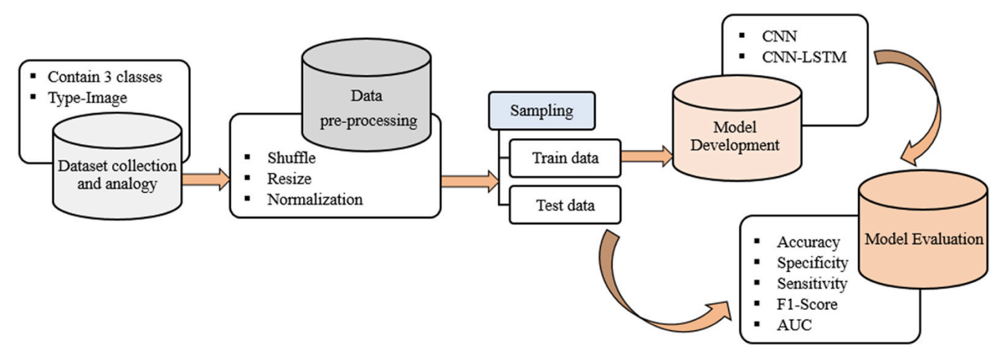
Figure 1. Overall system architecture. Raw chest X-rays are preprocessed (shuffle, resize, normalization), split into training/testing sets, and used to train both a baseline CNN and the proposed CNN-LSTM. Performance is evaluated using accuracy, specificity, sensitivity, F1-score, confusion matrix, and ROC/AUC.
📊 Dataset & Class Partition (Table 1, Fig. 2)
Because large labeled COVID-19 X-ray repositories were limited at the time, the dataset was assembled from multiple public sources. Images were resized to 224 × 224. The final dataset contains 4,575 X-rays with balanced classes: 1,525 COVID-19, 1,525 Normal, and 1,525 Pneumonia.
| Split | COVID-19 | Normal | Pneumonia | Overall |
|---|---|---|---|---|
| Training | 1220 | 1220 | 1220 | 3660 |
| Testing | 305 | 305 | 305 | 915 |
| Overall | 1525 | 1525 | 1525 | 4575 |
Table 1. Partitioning description of the used dataset.
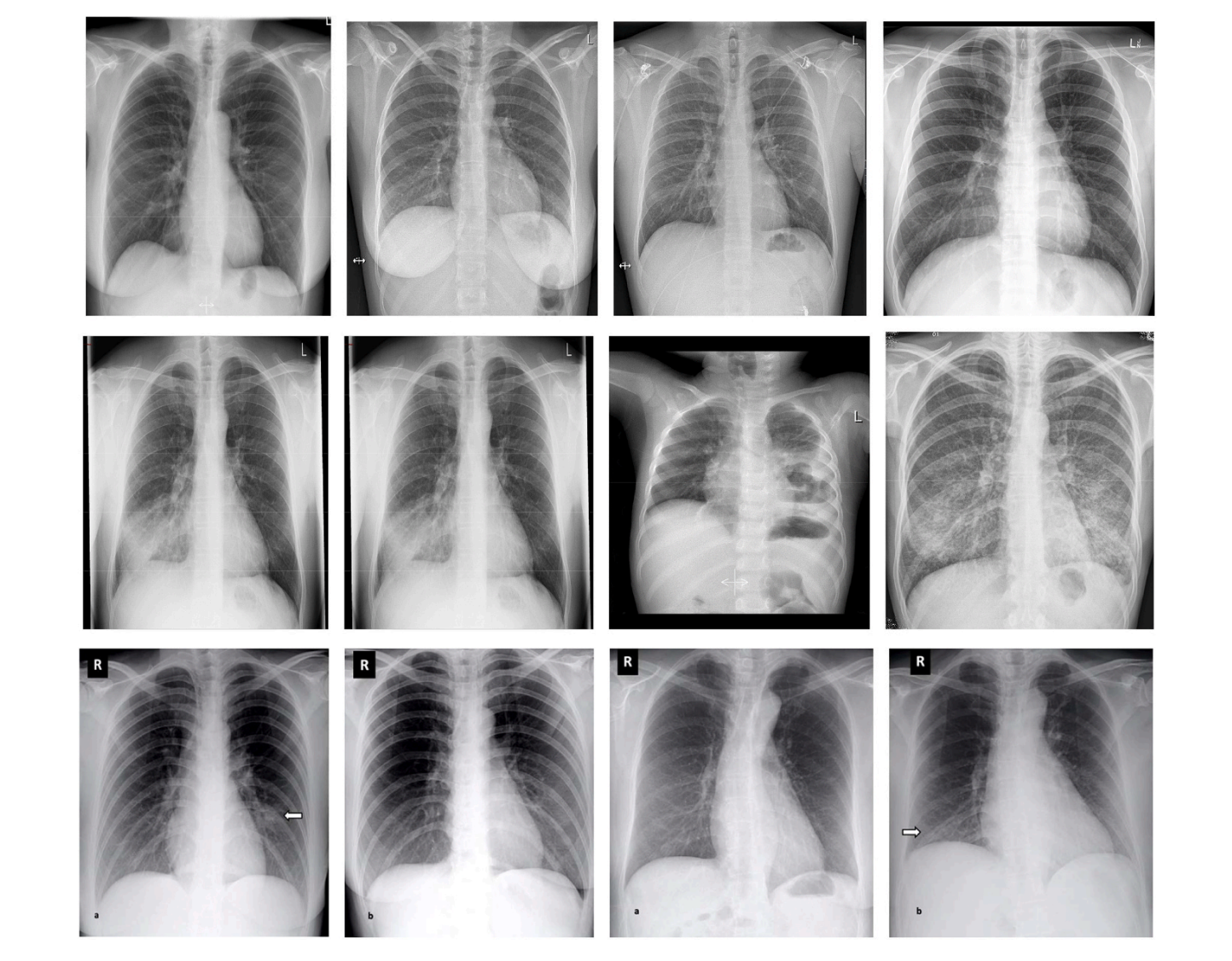
Figure 2. Sample images from each class. The paper shows example X-rays for COVID-19, Pneumonia, and Normal categories. :
🧠 Model Components (Figs. 3–5)
CNN Feature Extraction (Fig. 3)
- Core layers: Convolution → ReLU → Pooling → Fully Connected
- Goal: Learn hierarchical visual features from X-ray images
- Output: High-level feature maps passed to the classifier stage
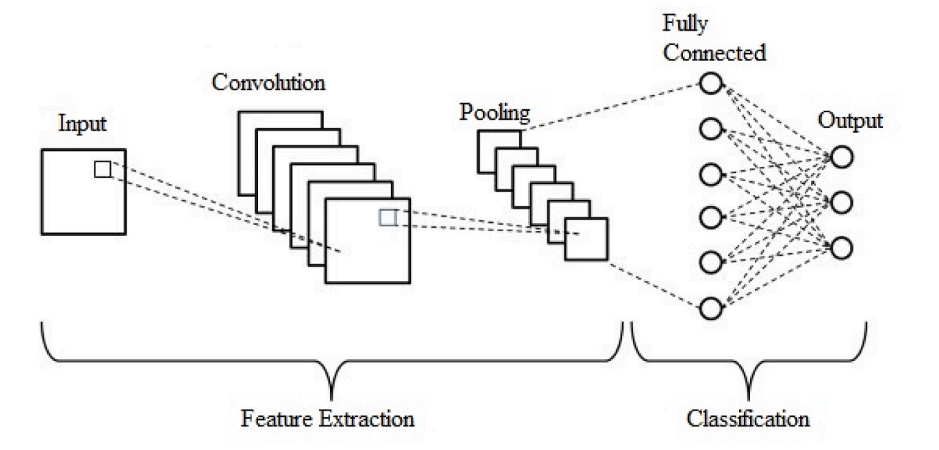
Figure 3. Typical CNN architecture (feature extraction + classification).
LSTM Classifier (Fig. 4)
- Motivation: LSTM is used as the classifier after CNN feature extraction
- Mechanism: Input/forget/output gates maintain and update memory state
- Paper focus: Explains LSTM equations and gate operations used in the model
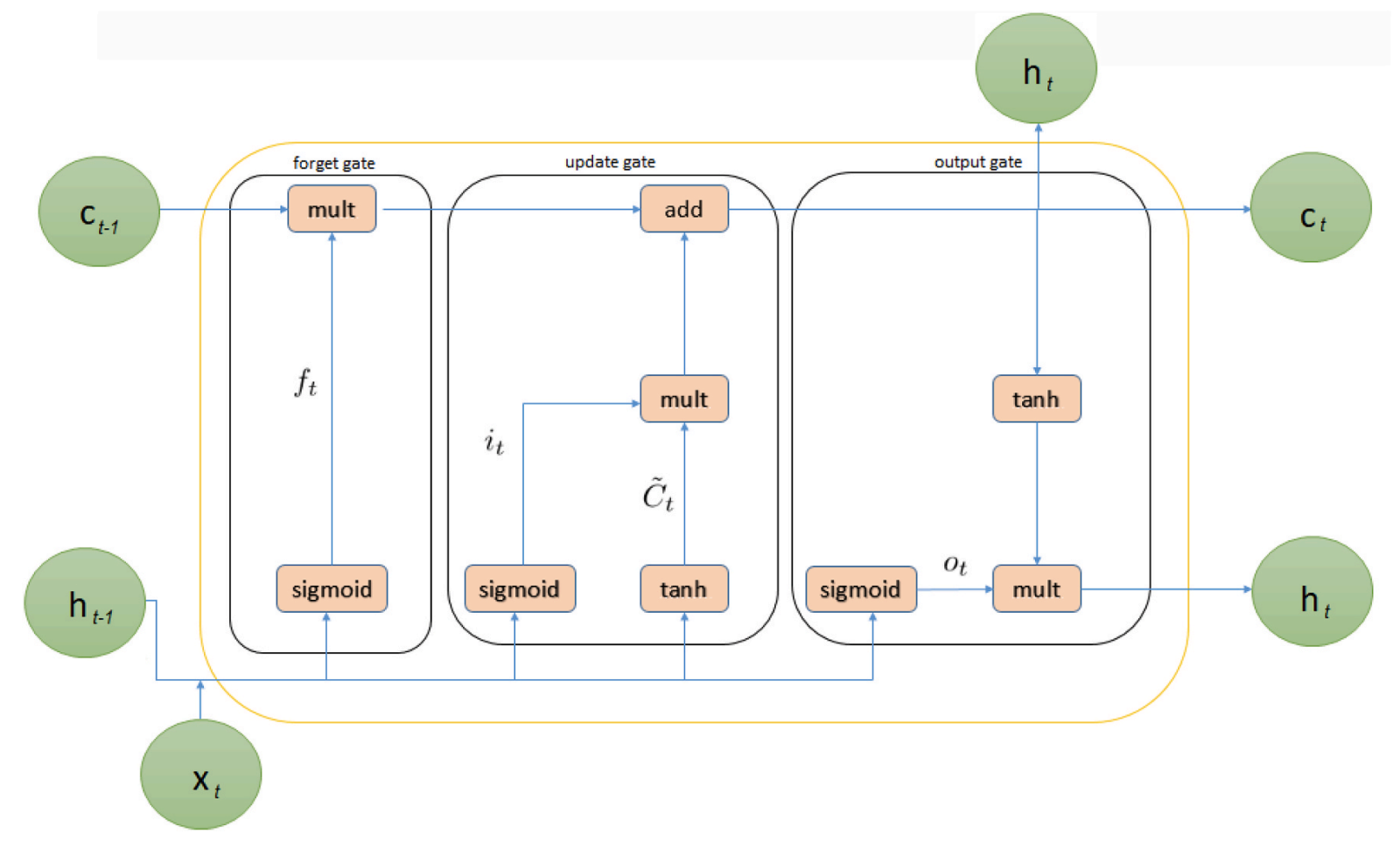
Figure 4. Internal structure of Long Short-Term Memory (LSTM).
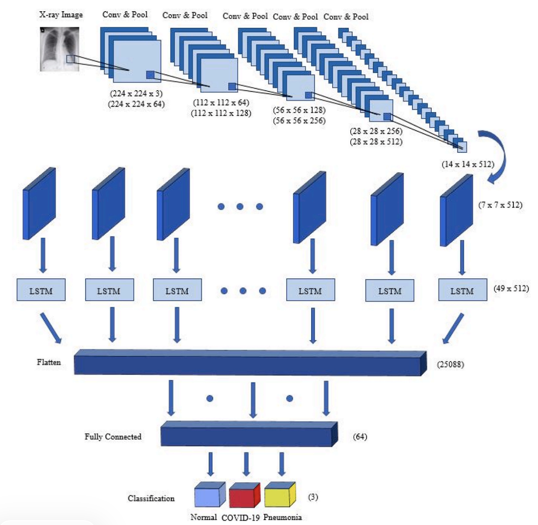
Figure 5. Proposed hybrid CNN-LSTM network. After multiple Conv+Pool blocks, the feature map shape becomes (7, 7, 512), reshaped to (49, 512) before entering the LSTM, then passed through a fully connected layer and softmax output for 3-class prediction.
📐 Full Architecture Summary (Table 2)
The proposed network has 20 layers: 12 convolution, 5 pooling, 1 LSTM, 1 fully connected, and 1 output (softmax). Dropout is applied after pooling with a 25% rate, and convolution uses 3×3 kernels with ReLU activation.
| Layer | Type | Kernel | Stride | #Kernels / Units | Input Size |
|---|---|---|---|---|---|
| 1 | Conv2D | 3×3 | 1 | 64 | 224×224×3 |
| 2 | Conv2D | 3×3 | 1 | 64 | 224×224×64 |
| 3 | Pool | 2×2 | 2 | – | 224×224×64 |
| 4–6 | Conv/Conv/Pool | 3×3, 3×3, 2×2 | 1, 1, 2 | 128, 128, – | 112×112×64 → 112×112×128 |
| 7–9 | Conv/Conv/Pool | 3×3, 3×3, 2×2 | 1, 1, 2 | 256, 256, – | 56×56×128 → 56×56×256 |
| 10–13 | Conv/Conv/Conv/Pool | 3×3, 3×3, 3×3, 2×2 | 1, 1, 1, 2 | 512, 512, 512, – | 28×28×256 → 28×28×512 |
| 14–17 | Conv/Conv/Conv/Pool | 3×3, 3×3, 3×3, 2×2 | 1, 1, 1, 2 | 512, 512, 512, – | 14×14×512 → 14×14×512 |
| 18 | LSTM | – | – | – | 49×512 |
| 19 | FC | – | – | 64 | 25,088 |
| 20 | Output | – | – | 3 | 64 |
Table 2. Full summary of the CNN-LSTM network (layer-by-layer).
🧪 Experimental Setup
- Train/Test split: 80% / 20% (training 3660, testing 915)
- Validation: 5-fold cross-validation
- Learning rate: 0.0001
- Epochs: 125
- Implementation: Python + Keras (TensorFlow2)
- Hardware: Intel Core i7 (2.2 GHz), NVIDIA GTX 1050 Ti (4 GB), 16 GB RAM
(All values above are reported in the paper’s experimental setup section.)
📈 Results & Analysis
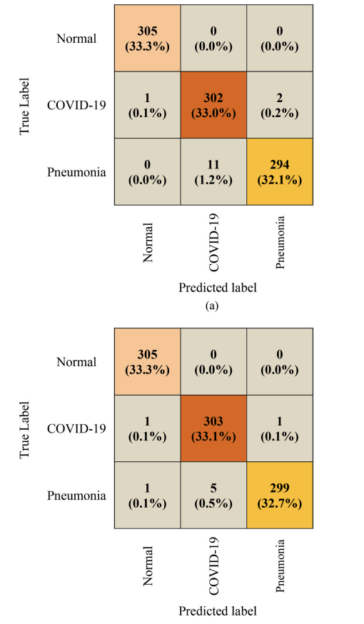
Figure 6. Confusion matrices. The paper compares baseline CNN vs proposed CNN-LSTM on the same 915-image test set, showing fewer misclassifications for CNN-LSTM.
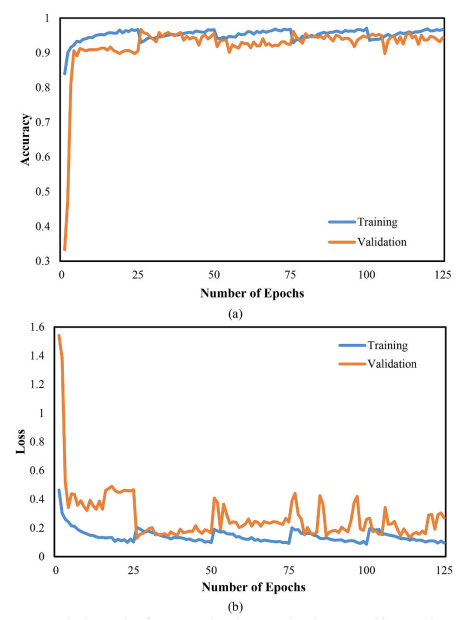
Figure 7. CNN training/validation accuracy and loss.
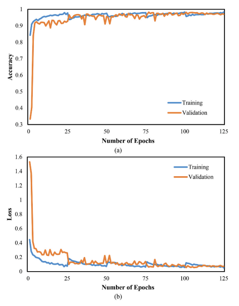
Figure 8. CNN-LSTM training/validation accuracy and loss.
📊 Quantitative Performance (Tables 3–5)
Baseline CNN Performance (Table 3)
| Class | Accuracy (%) | Specificity (%) | Sensitivity (%) | F1-Score (%) |
|---|---|---|---|---|
| COVID-19 | 98.5 | 98.2 | 99.0 | 97.7 |
| Pneumonia | 98.6 | 99.7 | 96.4 | 97.8 |
| Normal | 99.9 | 99.8 | 100.0 | 99.8 |
Table 3. Performance of the CNN network. :contentReference[oaicite:14]{index=14}
Proposed CNN-LSTM Performance (Table 4)
| Class | Accuracy (%) | Specificity (%) | Sensitivity (%) | F1-Score (%) |
|---|---|---|---|---|
| COVID-19 | 99.2 | 99.2 | 99.3 | 98.9 |
| Pneumonia | 99.2 | 99.8 | 98.0 | 98.8 |
| Normal | 99.8 | 99.7 | 100.0 | 99.7 |
Table 4. Performance of the CNN-LSTM network.
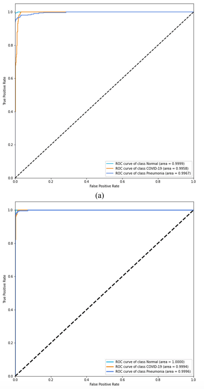
Figure 11. ROC analysis. The paper reports AUC ≈ 99.8% for CNN and ≈ 99.9% for CNN-LSTM, indicating stronger overall separability for the proposed model.
Comparison with Prior Work (Table 5)
The paper includes a comparison table across multiple published COVID-19 X-ray studies (accuracy and, when available, training/testing time), and reports the proposed CNN-LSTM as 99.4% overall accuracy with reported training/testing times of 18372.0 s / 113.0 s.
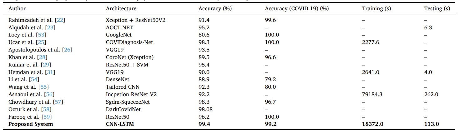
Table 5. Comparison of the proposed system with existing systems in terms of accuracy and computational time.
🩻 Interpretability: Grad-CAM Visual Explanations (Fig. 12)
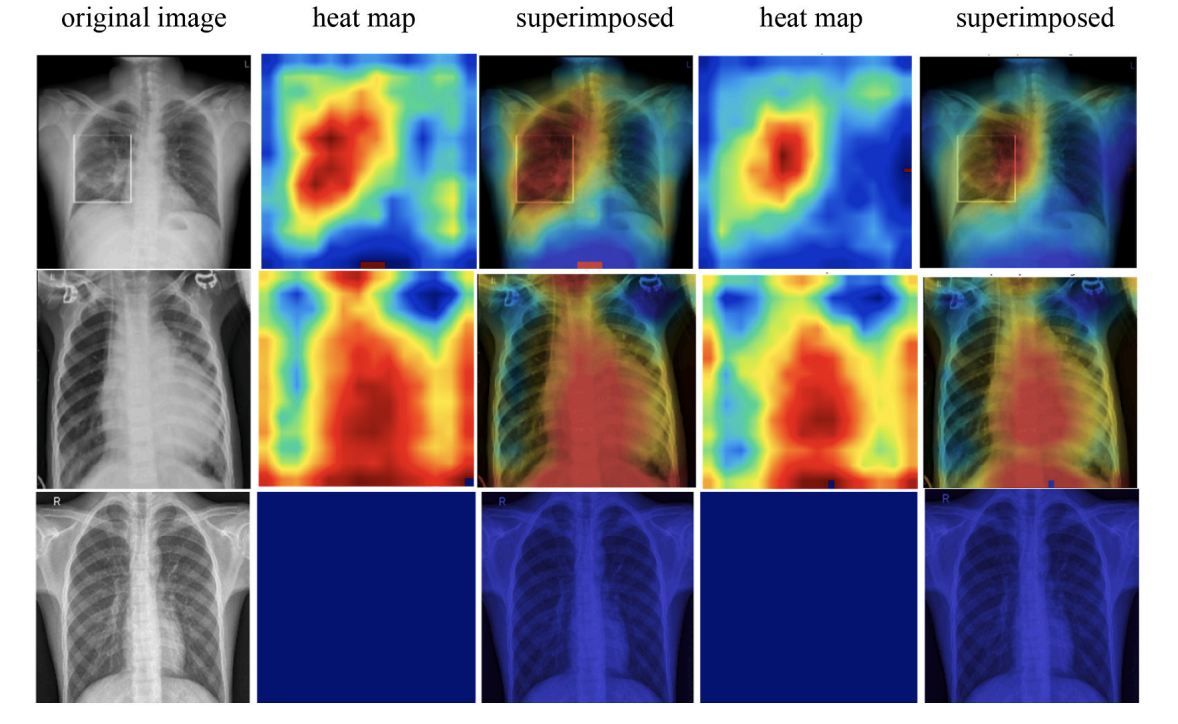
Figure 12. Grad-CAM heatmaps. The paper visualizes attention regions for COVID-19, Pneumonia, and Normal samples, showing heatmaps and superimposed views for both CNN and CNN-LSTM models.
🚀 Key Contributions & Practical Impact
Technical Contributions
- Hybrid design: CNN extracts deep spatial features; LSTM performs classification on reshaped features
- Balanced 3-class dataset: 1,525 images per class for COVID-19 / Normal / Pneumonia
- Full evaluation suite: Confusion matrix, ROC/AUC, accuracy/loss curves, and Grad-CAM interpretation
- Reproducible configuration: Learning rate 0.0001, 125 epochs, 5-fold cross-validation
Clinical / Deployment Notes (as stated in the paper)
- Goal: Assist clinicians by providing fast, consistent screening support from chest X-rays
- Limitations: Dataset size (generalizability), PA-view focus only, complex multi-symptom COVID-19 cases, and no radiologist comparison
- Future work: Increase sample size, support other X-ray views (AP/lateral), and compare with radiologists
🔬 Research Significance
This work demonstrates that combining CNN feature extraction with an LSTM classifier can achieve strong COVID-19 vs Pneumonia vs Normal discrimination on a balanced chest X-ray dataset, while also providing interpretability via Grad-CAM and reporting end-to-end experimental details. The paper also clearly states practical limitations and future directions needed for broader clinical validation. :contentReference[oaicite:20]{index=20}
📝 Citation
If you find CNN-LSTM paper useful in your research, please consider citing:
@article{islam2020combined,
  title={A combined deep CNN-LSTM network for the detection of novel coronavirus (COVID-19) using X-ray images},
  author={Islam, Md Zabirul and Islam, Md Milon and Asraf, Amanullah},
  journal={Informatics in medicine unlocked},
  volume={20},
  pages={100412},
  year={2020},
  publisher={Elsevier}
}Diagnosis of COVID-19 from X-rays using combined CNN-RNN architecture with transfer learning
Highlights
This paper proposes a combined CNN–RNN (LSTM) architecture with transfer learning to classify chest X-ray images into COVID-19, Pneumonia, and Normal. Four ImageNet-pretrained CNN backbones (VGG19, DenseNet121, InceptionV3, Inception-ResNetV2) are used for feature extraction, and a recurrent layer is used to classify the reshaped feature sequence. The study reports that VGG19-RNN achieves the best overall performance and visualizes decision regions with Grad-CAM.
Key Achievements (as reported in the paper):
- 🧠 Hybrid Transfer Model: Frozen pretrained CNN for feature extraction + single-layer recurrent classifier + FC + softmax
- 📦 Balanced 3-Class Dataset: 6,939 total X-rays; 2,313 per class (COVID-19 / Pneumonia / Normal)
- 🖼️ Standardized Input: Images resized to 224 × 224 × 3, shuffled and pixel-normalized
- ✅ Best Model: VGG19-RNN reported as top performer (overall accuracy 99.86%, AUC 99.99%)
- 📊 Evaluation Suite: Confusion matrix, Accuracy, Precision, Recall, F1, ROC curve, PR curve
- 🔥 Interpretability: Grad-CAM heatmaps + superimposed views for COVID-19 / Pneumonia / Normal
- ⚙️ Training Setup: RMSprop, batch size 32, learning rate 1e-5, 100 epochs, 5-fold cross-validation
- 🧾 Open Resources: Data and code links are provided by the authors in the paper
🏗️ Overall System Pipeline (Fig. 1)
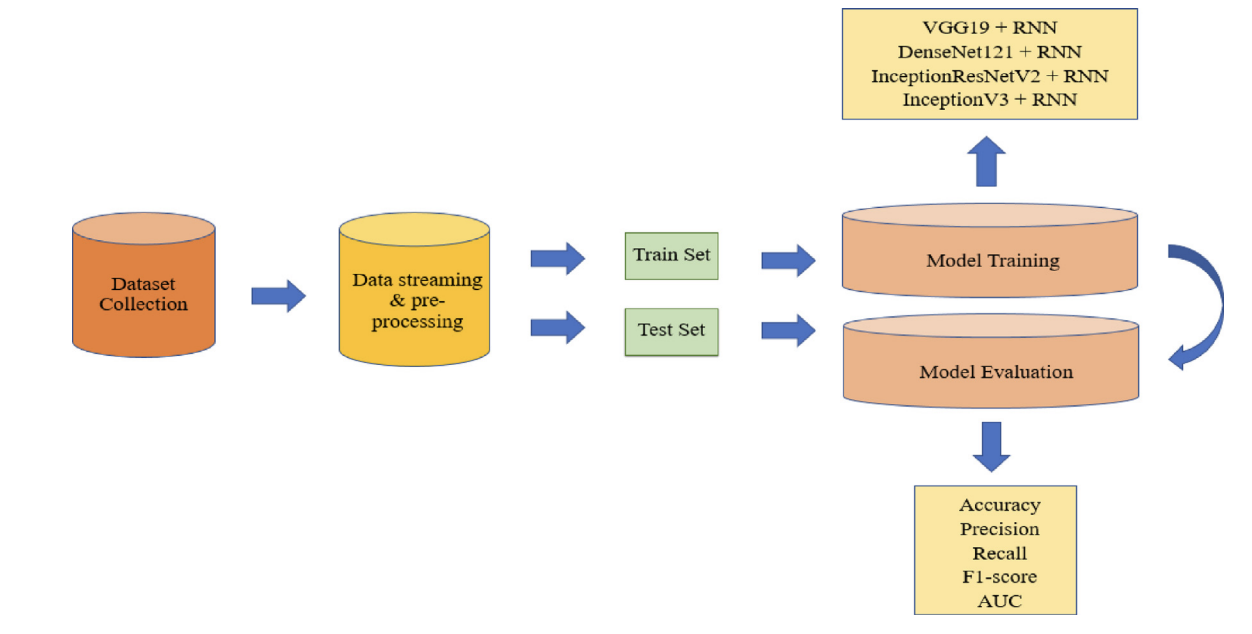
Figure 1. Overall system architecture of the COVID-19 diagnosis framework. The workflow starts with dataset collection and preprocessing (resize, shuffle, normalization), then splits data into train/test sets. Training evaluates four transfer-learning backbones (VGG19, DenseNet121, InceptionV3, Inception-ResNetV2) combined with a recurrent classifier. Performance is reported using Accuracy/Precision/Recall/F1/AUC and confusion matrices.
📊 Dataset & Class Partition (Table 1)
The paper constructs a balanced dataset by gathering COVID-19 X-rays from multiple public sources, and Pneumonia/Normal X-rays from Kaggle sources. The final dataset contains 6,939 images total: 2,313 COVID-19, 2,312 Pneumonia, and 2,313 Normal. An 80% / 20% train/test split is used, and the authors note that the test set contains only original images.
| Images | COVID-19 | Pneumonia | Normal | Total |
|---|---|---|---|---|
| Training | 1850 | 1851 | 1850 | 5551 |
| Testing | 463 | 462 | 463 | 1388 |
| Total | 2313 | 2312 | 2313 | 6939 |
Table 1. Dataset composition and train/test split used in the paper.
🧠 Transfer Learning Backbones (Table 2)
The authors compare four pretrained CNN architectures (ImageNet weights) as feature extractors. Their depths and parameter counts are summarized below.
| Network | Depth | Parameters (106) |
|---|---|---|
| VGG19 | 26 | 143.67 |
| DenseNet121 | 121 | 8.06 |
| InceptionV3 | 159 | 23.85 |
| Inception-ResNetV2 | 572 | 55.87 |
Table 2. Characteristics of the four pre-trained CNN architectures.
🔁 Recurrent Classifier Background (Fig. 2)
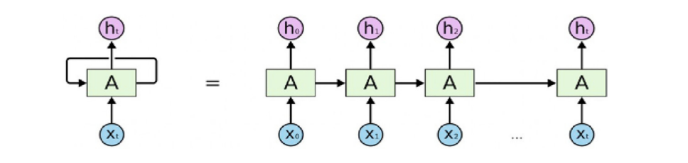
Figure 2. The structure of recurrent neural networks. The paper introduces RNNs for sequence modeling and motivates LSTM gating (input/forget/output gates) to handle long-term dependencies.
🧩 CNN–RNN Workflow (Fig. 3)
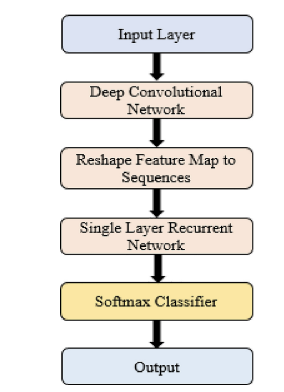
Figure 3. Workflow of the CNN-RNN architecture for COVID-19 diagnosis. A pretrained CNN extracts feature maps, the feature tensor is reshaped into a sequence, and a single recurrent layer processes the sequence before a softmax layer produces the final 3-class prediction.
🧠 Combined CNN–RNN Architecture (Fig. 4)
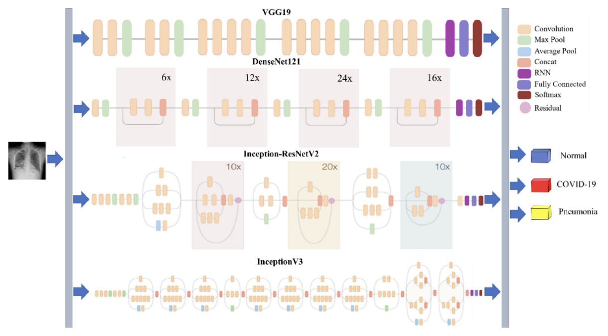
Figure 4. The structure of the combined CNN-RNN architecture for COVID-19 diagnosis. The figure summarizes the four backbone options feeding into the recurrent stage, followed by fully connected layers and a softmax output.
📐 Architecture Summary (Table 3)
The paper reports feature-map sizes and the reshape-to-sequence design for each backbone. Below is the architecture summary (Table 3 a–d), transcribed into HTML.
(a) VGG19-RNN
| Layer (type) | Input size | Output size |
|---|---|---|
| pretrained (VGG19) | 224, 224, 3 | 7, 7, 512 |
| reshape (Reshape) | 7, 7, 512 | 49, 512 |
| lstm (LSTM) | 49, 512 | 49, 512 |
| flatten (Flatten) | 49, 512 | 25088 |
| fc_1 (Dense) | 25088 | 4096 |
| fc_2 (Dense) | 4096 | 4096 |
| output (Dense) | 4096 | 3 |
(b) DenseNet121-RNN
| Layer (type) | Input size | Output size |
|---|---|---|
| pretrained (DenseNet121) | 224, 224, 3 | 7, 7, 1024 |
| reshape (Reshape) | 7, 7, 1024 | 49, 1024 |
| lstm (LSTM) | 49, 1024 | 49, 1024 |
| flatten (Flatten) | 49, 1024 | 50176 |
| fc_1 (Dense) | 50176 | 4096 |
| fc_2 (Dense) | 4096 | 4096 |
| output (Dense) | 4096 | 3 |
(c) Inception-ResNetV2-RNN
| Layer (type) | Input size | Output size |
|---|---|---|
| pretrained (Inception-ResNetV2) | 224, 224, 3 | 5, 5, 1536 |
| reshape (Reshape) | 5, 5, 1536 | 25, 1536 |
| lstm (LSTM) | 25, 1536 | 25, 512 |
| flatten (Flatten) | 25, 512 | 12800 |
| fc_1 (Dense) | 12800 | 4096 |
| fc_2 (Dense) | 4096 | 4096 |
| output (Dense) | 4096 | 3 |
(d) InceptionV3-RNN
| Layer (type) | Input size | Output size |
|---|---|---|
| pretrained (InceptionV3) | 224, 224, 3 | 5, 5, 2048 |
| reshape (Reshape) | 5, 5, 2048 | 25, 2048 |
| lstm (LSTM) | 25, 2048 | 25, 512 |
| flatten (Flatten) | 25, 512 | 12800 |
| fc_1 (Dense) | 12800 | 4096 |
| fc_2 (Dense) | 4096 | 4096 |
| output (Dense) | 4096 | 3 |
Table 3. Summary of the used architectures (a–d).
🧪 Experimental Setup
- Platform: Google Colaboratory Linux (Ubuntu 16.04)
- GPU: Tesla K80
- Framework: Python (TensorFlow/Keras)
- Optimization: RMSprop
- Batch size: 32
- Learning rate: 1e-5
- Epochs: 100
- Validation: 5-fold cross-validation
- Training policy: Pretrained CNN layers frozen; recurrent + FC layers trained; dropout used to reduce overfitting
📈 Results & Analysis
Training & Validation Curves (Fig. 5)
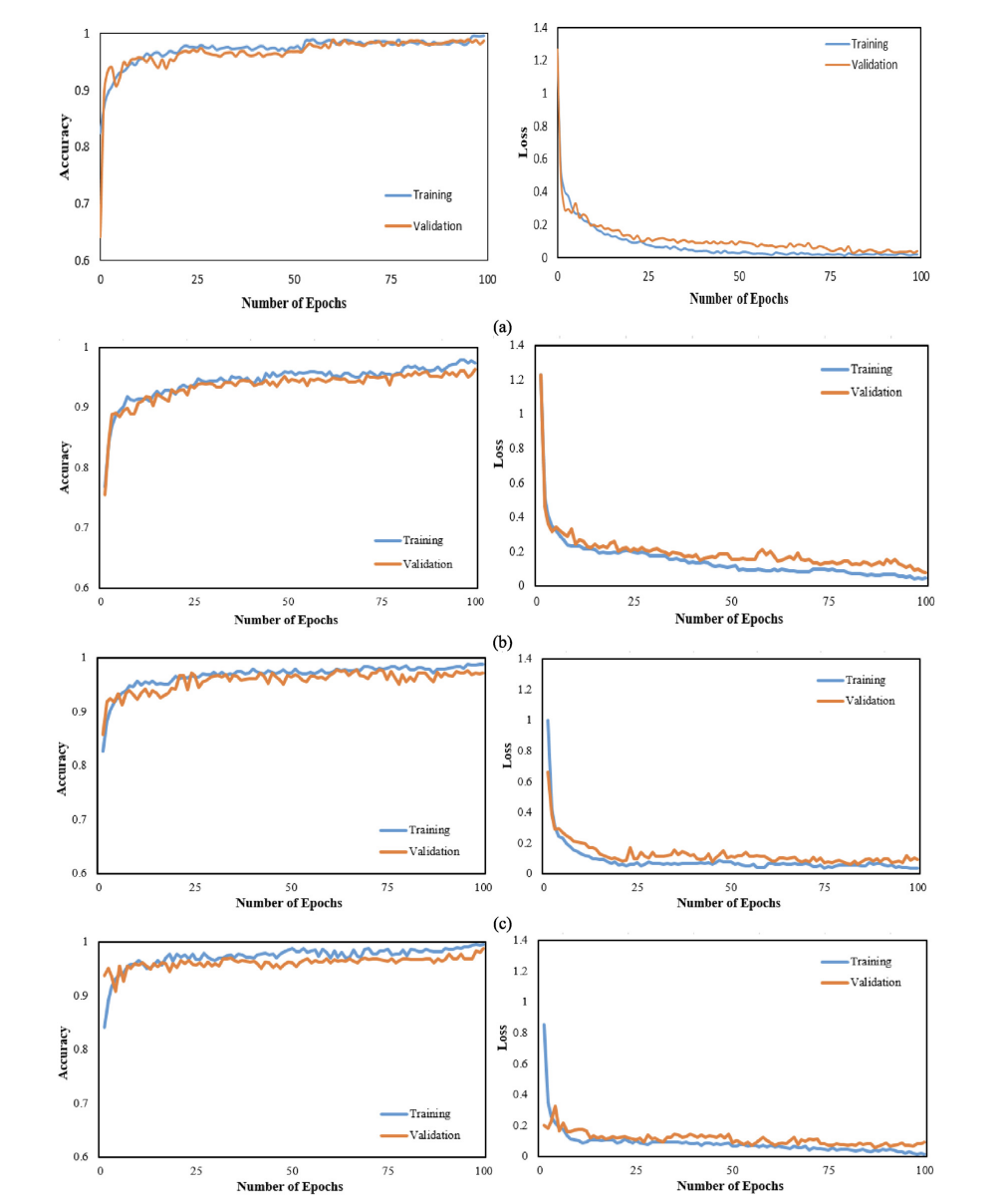
Figure 5. Accuracy and loss curves for all four CNN-RNN architectures (VGG19, DenseNet121, InceptionV3, Inception-ResNetV2).
Confusion Matrices (Fig. 6)
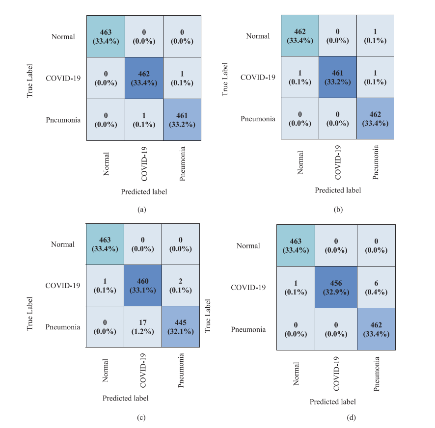
Figure 6. Confusion matrices for the four architectures on the 1,388-image test set.
Computational Time Comparison (Table 4)
| Model | Training time (s) | Testing time (s) |
|---|---|---|
| VGG19 | 16722.41 | 129.69 |
| DenseNet121 | 18145.67 | 196.02 |
| InceptionV3 | 16376.09 | 170.14 |
| Inception-ResNetV2 | 17727.26 | 310.63 |
Table 4. Comparative computational time for the CNN-RNN models.
Main Quantitative Performance (Table 5: COVID-19 row shown)
| Classifier | Patient status | AUC (%) | Accuracy (%) | Precision (%) | Recall (%) | F1-score (%) |
|---|---|---|---|---|---|---|
| VGG19-RNN | COVID-19 | 99.99 | 99.86 | 99.78 | 99.78 | 99.78 |
| DenseNet121-RNN | COVID-19 | 99.99 | 99.78 | 99.57 | 100.0 | 99.78 |
| InceptionV3-RNN | COVID-19 | 99.95 | 98.56 | 99.35 | 96.44 | 97.87 |
| Inception-ResNetV2-RNN | COVID-19 | 99.99 | 99.50 | 98.49 | 100.0 | 99.24 |
Table 5. Performance of the combined CNN-RNN architectures (COVID-19 row shown; the paper includes all classes).
🩻 Interpretability with Grad-CAM (Fig. 9)
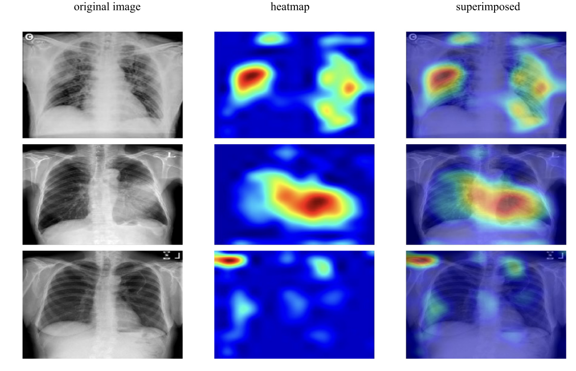
Figure 9. Grad-CAM visualizations for VGG19-RNN to highlight class-relevant regions in chest X-rays.
⚠️ Limitations & Future Directions (as stated)
- Dataset growth: The paper notes that larger COVID-19 collections would strengthen validation.
- View generalization: Experiments focus on PA chest X-rays and may not generalize to other views.
- Clinical comparison: Future work includes comparing model performance against radiologists.
📝 Citation
If you find CNN-RNN paper useful in your research, please consider citing:
@article{islam2022diagnosis,
  title={Diagnosis of COVID-19 from X-rays using combined CNN-RNN architecture with transfer learning},
  author={Islam, Md Milon and Islam, Md Zabirul and Asraf, Amanullah and Al-Rakhami, Mabrook S and Ding, Weiping and Sodhro, Ali Hassan},
  journal={BenchCouncil Transactions on Benchmarks, Standards and Evaluations},
  volume={2},
  number={4},
  pages={100088},
  year={2022},
  publisher={Elsevier}
}Deep Learning Applications to Combat Novel Coronavirus (COVID-19) Pandemic
Highlights
During the COVID-19 pandemic, deep learning has been explored across the full response pipeline, not only for diagnosis from medical images, but also for disease tracking, protein structure prediction, drug discovery, and understanding virus severity and infectivity. This review summarizes representative studies in each area, discusses current constraints (including data limitations and interpretability gaps), and outlines directions for future work.
Key Takeaways (as stated in the paper):
- 🩻 Diagnosis via imaging: Deep learning on X-ray and CT has been widely studied for COVID-19 screening and differentiation from other lung diseases.
- 🗺️ Disease tracking: Deep learning applied to real-time signals and time series helps forecast trends and estimate risk.
- 🧬 Protein structure: Deep models (e.g., AlphaFold-style approaches) support structure prediction that may inform downstream drug/vaccine research.
- 💊 Drug discovery: Generative models and reinforcement learning are explored to generate or repurpose candidate compounds.
- 🦠 Severity & infectivity: Sequence-based deep learning is used for virus-host prediction and infectivity assessment.
- ⚠️ Challenges: Limited COVID-19 data, varying reporting quality, and insufficient interpretability/transparency are recurring issues.
🧭 Scope of the Review
The review organizes deep learning contributions into five main application directions: (1) medical imaging for diagnosis, (2) disease tracking, (3) protein structure prediction, (4) drug discovery, and (5) virus severity and infectivity. It also summarizes constraints and future directions for real-world deployment.
🏗️ Deep Learning Applications for COVID-19 (Fig. 1)
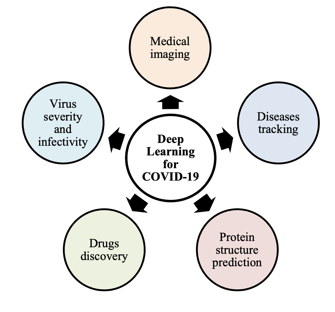
Figure 1. Deep learning applications for COVID-19 pandemic. The paper highlights five major dimensions where deep learning has been used: medical imaging, disease tracking, protein structure prediction, drug discovery, and virus severity/infectivity.
🩻 Medical Imaging for Diagnosis
The paper notes that RT-PCR is a key diagnostic indicator but is time-consuming and can have a high false-negative rate. As a complementary approach, deep learning has been applied to chest X-ray and CT for COVID-19 detection and for differentiating COVID-19 pneumonia from other conditions.
Examples discussed include COVID-Net on X-rays, modified Inception-style transfer learning on CT, 3D deep learning with location-attention mechanisms, and architectures combining CNNs with attention modules. The paper also includes a study using a combined CNN-LSTM approach on X-rays.
📊 Summary of Imaging-Based Diagnosis Works (Table 1)
| Authors | Sample size | Methods | Results |
|---|---|---|---|
| Khan et al. | 1300 chest X-rays including 290 COVID-19 cases | CoroNet: Xception architecture | Accuracy = 89.6% |
| Wu et al. | 495 CT images consisting of 368 COVID-19 cases | Multi-view fusion model using deep learning techniques | Accuracy = 70.0%; AUC = 73.2% |
| Wang and Wong | 13,975 X-ray images from 13,870 patients | COVID-Net: deep CNN architecture | Accuracy = 92.4% |
| Wang et al. | 325 CT scans of COVID-19 and 740 of pneumonia | Deep transfer learning using modified Inception | Accuracy = 79.3%; Specificity = 83.0% |
| Butt et al. | 618 CT images including 219 COVID-19 cases | 3D deep learning with location-attention mechanism | Accuracy = 86.7% |
| Jin et al. | 970 CT images from 496 patients | Deep neural network | Accuracy = 94.98%; Specificity = 95.47% |
| Song et al. | 275 CT scans comprising of 88 COVID-19 cases | DeepPneumonia: ResNet architecture | AUC = 99.0%; Sensitivity = 93.0% |
| Islam et al. | 421 X-ray images including 141 COVID-19 cases | Combined deep CNN-LSTM architecture | Accuracy = 97%; Specificity = 91% |
Table 1. Summarization of deep learning applications for medical imaging-based COVID-19 diagnosis.
🗺️ Disease Tracking
The review discusses deep learning for tracking outbreak dynamics using multiple signal sources. Examples include using deep models to analyze respiratory patterns (e.g., tachypnea screening from depth camera signals), smartphone sensor–based symptom detection, community-level risk assessment using real-time data, and time series forecasting using recurrent architectures such as LSTM/GRU.
🧬 Protein Structure Prediction
The paper describes protein structure prediction as an important step in understanding viral mechanisms and supporting drug/vaccine development. It contrasts template modeling and template-free modeling, and highlights deep neural approaches (including ResNet-style models used in AlphaFold-like systems) for predicting 3D protein structures. The review notes such predictions still require experimental verification.
💊 Drug Discovery
The review summarizes deep learning approaches to identify candidate drugs for COVID-19, including: (i) generative modeling pipelines (e.g., generative auto-encoders and GANs) to propose inhibitors, (ii) reinforcement learning (e.g., deep Q-learning) for fragment-based drug design, and (iii) drug–target interaction models for repurposing existing antivirals. The paper also cautions that limited data can introduce training errors.
🦠 Virus Severity and Infectivity
The paper highlights deep learning for viral host prediction and infectivity assessment using genomic sequence data. It notes CNN/LSTM-based models can outperform traditional machine learning baselines in some settings, and that interpretability tools (e.g., visualization of sequence patterns) can help analyze model behavior.
📌 Overall Summary of Deep Learning Applications (Table 2)
| Sl. no. | Applications | Descriptions |
|---|---|---|
| 1 | Diagnosis using medical imaging | Deep learning is used to extract complex features from radiological images for diagnosis. Examples include CNN-based screening from increasing samples, Xception-based CoroNet on X-rays, COVID-Net on X-rays, and ResNet-based approaches (e.g., DeepPneumonia) on CT scans. |
| 2 | Disease tracking | Models such as bidirectional GRU with attention for respiratory pattern analysis; neural networks for geographic spread; deep learning on real-time data for community-level risk; and outbreak forecasting with recurrent networks (e.g., LSTM). |
| 3 | Protein structure prediction | Deep neural methods for predicting protein structure and characteristics, including CNN-style dense prediction and deeper ResNet-style networks to ease training for recognition tasks; supports understanding and vaccine-related research. |
| 4 | Drug discovery | Generative models (GANs/GAs) to generate candidate compounds; reinforcement learning to discover inhibitors; and deep models to generate new molecules and evaluate protein–ligand interactions. |
| 5 | Virus severity and infectivity | Sequence-based CNN/LSTM models for predicting virus infectivity in humans; virus-host prediction with deep learning to support early analysis and prevention. |
Table 2. Summarization of deep learning applications to combat COVID-19 pandemic.
🧩 Discussion: Constraints, Challenges, and What’s Missing
- Limited and uneven data: The paper emphasizes that COVID-19 data was limited, and that case reporting can vary across countries, which can affect disease tracking and modeling.
- Interpretability gap in imaging: The review notes that some imaging-based deep learning systems lack transparency, making it unclear which imaging features drive predictions. It argues that explaining feature evidence could help clinicians gain insight.
- Drug discovery complexity: The paper notes needs such as longer peptides in virtual screening and improved scoring functions for antibody redesign, and highlights that limited training data can introduce errors.
✅ Conclusion
The paper concludes that deep learning can contribute at multiple levels (medical imaging, molecular biology, epidemiology) for early identification, outbreak monitoring, and accelerating drug/vaccine-related research. At the same time, it stresses that real-world impact is constrained by data availability and the need for stronger transparency and validation.
📝 Citation
If you find this paper useful in your research, please consider citing:
@article{asraf2020deep,
  title={Deep learning applications to combat novel coronavirus (COVID-19) pandemic},
  author={Asraf, Amanullah and Islam, Md Zabirul and Haque, Md Rezwanul and Islam, Md Milon},
  journal={SN Computer Science},
  volume={1},
  number={6},
  pages={363},
  year={2020},
  publisher={Springer}
}
📖 Paper:
SN Computer Science
Analyzing the Dynamics of COVID-19 Lockdown Success: Insights from Regional Data and Public Health Measures
Highlights
This paper analyzes why COVID-19 lockdowns succeeded in some regions and failed in others by building a 10,000-entry regional dataset (up to December 2022) across 100 countries. The study examines relationships among population density, infected, deaths, recovered, and a binary lockdown success/failure indicator. It uses three correlation approaches (Pearson, Spearman, Kendall) to quantify which variable pairs move together most strongly and suggests practical directions for managing future pandemics.
Key Contributions (as stated in the paper):
- 🧾 Comprehensive dataset: Built a multi-attribute COVID-19 dataset (regional area, population, infected, deaths, recovered, success/failure) with 10,000 entries from 100 countries.
- 📌 Added derived attribute: Computed population density from population and area and included it as an additional feature.
- 📐 Correlation analysis: Used Pearson’s r, Spearman’s rho, and Kendall’s tau to analyze inter-factor relationships.
- 🔎 Lockdown success insight: Visual analysis suggests lockdown success occurs more often in lower-density regions, with exceptions where strict measures were enforced.
- 🧭 Future directions: Proposes practical prevention strategies (e.g., social distancing, remote work, decentralized living) to reduce transmission risk.
🏗️ Overall System Pipeline (Fig. 1)
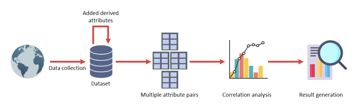
Figure 1. Overall architecture of the proposed framework. The workflow collects regional COVID-19 data, adds derived attributes (notably density), forms multiple attribute pairs, performs correlation analysis, and generates results about factor relationships and lockdown success.
📊 Dataset, Features & Preprocessing (Tables I–II)
The dataset is manually constructed with 10,000 records from 100 countries (up to December 2022). The original dataset contains 7 attributes: region name, infected, deaths, recovered, area, population, and lockdown success/failure. The authors then derive density = population / area, and encode success as 1 and failure as 0. To reduce bias, the dataset is balanced with 5,000 successes and 5,000 failures. Numeric attributes are normalized with min-max normalization to the range [0, 1].
Table I. Sample Dataset
| Region Name | Infected | Deaths | Recovered | Area | Population | Success/Failure |
|---|---|---|---|---|---|---|
| Alaska | 761 | 12 | 491 | 665384 | 731545 | success |
| Iowa | 28819 | 709 | 22870 | 56272 | 3155070 | failure |
| New York | 393454 | 24855 | 70590 | 54554 | 19453561 | failure |
| Maharashtra | 284281 | 11194 | 158140 | 307713 | 112374333 | success |
| North Dakota | 3313 | 77 | 2952 | 70698 | 762062 | success |
Table I. Sample dataset (7 features) as shown in the paper.
Table II. Derived Dataset (with Density and Binary Success)
| Region Name | Infected | Death | Recovered | Area | Population | Success/Failure | Density |
|---|---|---|---|---|---|---|---|
| Alaska | 761 | 12 | 491 | 665384 | 731545 | 1 | 1.0994 |
| Iowa | 28819 | 709 | 22870 | 56272 | 3155070 | 0 | 56.0682 |
| New York | 393454 | 24855 | 70590 | 54554 | 19453561 | 0 | 356.5927 |
| Maharashtra | 284281 | 11194 | 158140 | 307713 | 112374333 | 1 | 356.1920 |
| North Dakota | 3313 | 77 | 2952 | 70698 | 762062 | 1 | 10.7791 |
Table II. Derived dataset (adds Density and binary Success/Failure) as shown in the paper.
📐 Correlation Methods Used (Pearson, Spearman, Kendall) + Fig. 2
The paper uses three correlation coefficients to capture different relationship types: Pearson’s r (linear association), Spearman’s rho (rank-based monotonic association), and Kendall’s tau (rank-based dependence via concordant/discordant pairs).
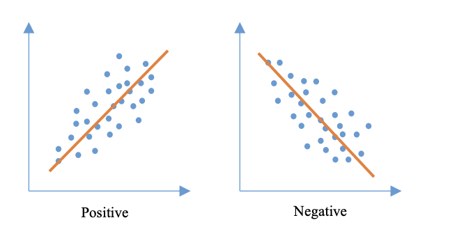
Figure 2. Types of correlation. The paper illustrates positive vs. negative correlation using example scatter plots and fitted trend lines.
🧪 Experimental Setup
- Platform: Kaggle online environment
- Language: Python
- Machine: Windows 11 desktop, Intel Core i5 @ 3.10 GHz, 12 GB RAM
- Parallel processing: Not used
🧾 Experimental Measurements (6 Attribute Pairs)
From the dataset attributes, the experiments focus on six pairwise combinations:
- (Density, Infected)
- (Density, Death)
- (Density, Recovered)
- (Death, Recovered)
- (Infected, Death)
- (Infected, Recovered)
📉 Scatter Plots of the 6 Pairs (Fig. 3)
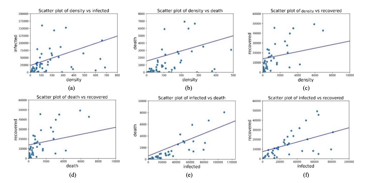
Figure 3. Scatter plot of (a) Density vs Infected, (b) Density vs Death, (c) Density vs Recovered, (d) Death vs Recovered, (e) Infected vs Death, and (f) Infected vs Recovered. The paper notes positive trends visually, then quantifies strength using correlation coefficients.
📊 Correlation Results (Tables III–V)
The paper reports correlation strength for the six attribute pairs using Pearson’s r, Spearman’s rho, and Kendall’s tau.
Table III. Pearson’s Correlation Coefficient
| Combination | Value of r | Strength (as labeled) |
|---|---|---|
| Density vs Infected | 0.384 | Moderate |
| Density vs Death | 0.284 | Weak |
| Density vs Recovered | 0.277 | Weak |
| Death vs Recovered | 0.412 | Moderate |
| Infected vs Death | 0.649 | Moderate |
| Infected vs Recovered | 0.755 | Strong |
Table III. Pearson correlation results for the six attribute pairs.
Table IV. Spearman’s Correlation Coefficient
| Combination | Value of r | Strength (as labeled) |
|---|---|---|
| Density vs Infected | 0.54 | Moderate |
| Density vs Death | 0.44 | Moderate |
| Density vs Recovered | 0.42 | Moderate |
| Death vs Recovered | 0.724 | Strong |
| Infected vs Death | 0.864 | Strong |
| Infected vs Recovered | 0.877 | Strong |
Table IV. Spearman correlation results for the six attribute pairs.
Table V. Kendall’s Correlation Coefficient
| Combination | Value of r | Strength (as labeled) |
|---|---|---|
| Density vs Infected | 0.413 | Moderate |
| Density vs Death | 0.347 | Weak |
| Density vs Recovered | 0.318 | Weak |
| Death vs Recovered | 0.582 | Moderate |
| Infected vs Death | 0.744 | Strong |
| Infected vs Recovered | 0.737 | Strong |
Table V. Kendall correlation results for the six attribute pairs.
🏘️ Effect of Density on Lockdown Success (Fig. 4)
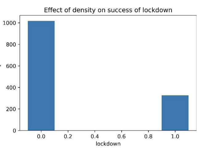
Figure 4. Effect of density on success of lockdown. The paper states that success is mostly observed in regions with lower population density, while some high-density regions still succeed when strict precautionary measures are implemented (e.g., daily goods and medicine supply, rule enforcement, and reduced social engagement).
✅ Key Findings & Practical Directions
What the correlations imply (in plain English)
- Infected vs Death and Infected vs Recovered show the strongest positive correlations (especially under Spearman and Kendall), meaning as infections rise, deaths and recoveries rise too.
- Pairs involving density tend to be weaker or moderate, which the paper interprets as density having a smaller direct association with infected/death/recovered compared to the infection–outcome relationships.
- Separately, the lockdown success visualization suggests density relates to whether lockdowns succeed, but it is not the only factor: strict public health and supply measures can still produce success in dense regions.
Proposed directions for future pandemics (as discussed)
- Reduce transmission opportunities: strengthen social distancing and reduce close-contact mixing.
- Reduce effective density during outbreaks: promote remote work and decentralized living arrangements when feasible.
- Support compliance: ensure supplies of daily necessities and medicines so restrictions remain practical.
🏁 Conclusion (Section V)
The paper concludes that using a multi-region dataset and multiple correlation measures can reveal meaningful relationships among COVID-19 factors. It reports strong positive correlations between infections and both deaths and recoveries, and highlights that lockdown success is often associated with lower density (with important real-world exceptions). The authors note limitations in data availability/quality and suggest expanding the dataset and experimental measurements in future work.
📝 Citation
If you find this paper useful in your research, please consider citing:
@article{manik2024analyzing,
  title={Analyzing the dynamics of covid-19 lockdown success: Insights from regional data and public health measures},
  author={Manik, Md Motaleb Hossen and Habib, Md Ahsan and Islam, Md Zabirul and Ahmed, Tanim and Haque, Fabliha},
  journal={arXiv preprint arXiv:2402.18594},
  year={2024}
}
📖 Paper:
arXiv preprint